How to Stream a Fantasy Football Kicker (Part 2 of 3)

How to Stream a Fantasy Football Kicker is a three-part series, and you’re currently reading Part 2 of 3. If you haven’t read Part 1 yet, I highly recommend starting there. It covers the basics you’ll need to make sense of what’s coming next. Click the blue button below to catch up.
How to Stream a Fantasy Kicker (Part 1 of 3)Also, all three parts of this series are built on my 2013 post, Using the Science of Statistics to Select a Fantasy Kicker. Think of it as the ancient scroll that started it all – the foundation for everything we’re doing here. Click the blue button below to check out the original post and see where it all began.
Using Statistics to Select a Fantasy KickerQuick Recap of Part 1
In the first post, I explained how fantasy football owners can gain an edge by streaming kickers, rotating them weekly based on matchup potential and using Las Vegas odds instead of traditional rankings.
Instead of focusing on traits like leg strength or accuracy, which have little correlation with a kicker’s fantasy success, the key is to target kickers from teams that Vegas expects to score the most points, since those teams tend to produce the best fantasy kicker results.
While this whole process may look a bit heady and intimidating at first, it’s actually easier than assembling IKEA furniture without cussing. By applying simple math to point spreads and over/under totals, you can quickly estimate each team’s projected points and make smarter weekly kicker choices.
What You’ll Learn in Part 2
In this post, I’ll show you how to streamline the entire process using Excel, allowing you to quickly find the best kicker options each week without doing all the math manually.
You’ll be copying Vegas odds from a website and pasting them into an Excel spreadsheet that automatically calculates projected team points and ranks every team accordingly.
Once the spreadsheet is built, it can be reused every week during the season. The steps are explained in detail so that anyone, no matter how comfortable you are with computers, can follow along successfully.
A Note Before We Begin
Although this process is much easier than folding a fitted bed sheet, if it still feels overwhelming, you might want to wait for Part 3. That section explains how to use AI to automatically create your kicker spreadsheet and happens to be the same method I use each week.
If you’re ready to give it a whirl, though, let’s roll up our sleeves and dive into the Excel approach.
Step 1: Create the Excel Spreadsheet
- Open Excel and start a new blank workbook.
Save it with a filename of your choice. (I used Kicker2025.xlsx.) Keep the file somewhere you can easily find later. - Set up your first worksheet (Sheet1).
In row 1, create five column headers:
o A1: RANK
o B1: TEAM
o C1: SPREAD
o D1: O/U
o E1: PROJ PTS - Add formulas.
o In cell A2, enter: =RANK(E2,E$2:E$33,0)
o Leave B2, C2, and D2 blank.
o In cell E2, enter: =(D2/2)-(C2/2) - Copy row 2 down through row 33 (for a total of 32 rows – one for each NFL team). To do this, select row 2, copy (Ctrl+C), then highlight rows 3–33 and paste (Ctrl+P).
When finished, your spreadsheet should look like Image 1. Save your file.
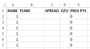
Image 1
Step 2: Add a Second Worksheet
By default, your new workbook only includes one worksheet named Sheet1.
Click the New Sheet (+) button at the bottom to add another and name it Sheet2.
Your spreadsheet should now have two worksheets: one sheet for your formulas (Sheet1) and one for your raw data (Sheet2). Save your progress.
Step 3: Get the Vegas Odds
Next, you’ll need a source for current NFL point spreads and over/unders.
The site I recommend is:
https://gridirongames.com/nfl-weekly-betting-lines/
Make sure the correct NFL week is displayed using the dropdown box above the odds table.
Now, referring to Image 2 for guidance…
- Start your mouse click just before the first team abbreviation (for example, BAL). This is marked with an A in the image.
- While holding the left mouse button, drag down to highlight all teams through the end of the final over/under total, which is marked with B. (In my example image, B isn’t shown at the very end of the data – I shortened the example for clarity – but when you do this step yourself, your B will be at the end of the final line of information in the full odds table. I hope that makes sense!)
- When everything is highlighted, copy it to your clipboard (Ctrl+C).
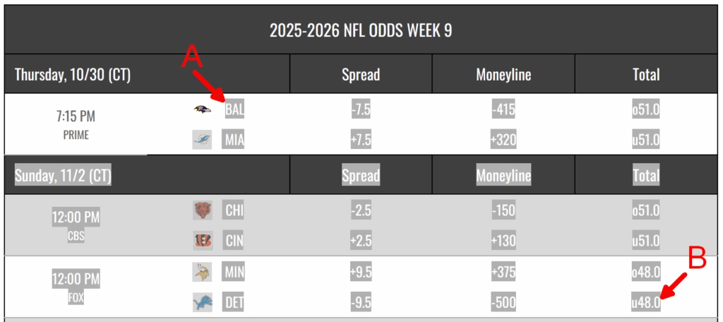
Image 2
Step 4: Clean Up the Data in Notepad
- Open Notepad and paste the copied text (Ctrl+P).
- You’ll see a mix of team abbreviations, odds, and descriptive text.
- Referring to Image 3, delete all of the yellow-highlighted descriptive information and keep only the green-highlighted team and odds data.
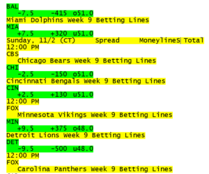
Image 3
When done, your Notepad file should look like Image 4: clean, simple, and ready for Excel.
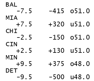
Image 4
Now highlight everything in Notepad, copy it (Ctrl+C), and switch back to Excel.
Step 5: Paste Odds into Sheet 2
- Go to Sheet2 and click cell A1.
- Paste (Ctrl+P) the contents from Notepad.
At this stage, your spreadsheet should resemble Image 5: team abbreviations listed on one row, with the corresponding Spread, Moneyline, and Over/Under totals listed on the line below.
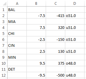
Image 5
We need to shift the odds up so each team’s data is on the same line. Highlight the odds columns (B through D) and move them up one row.
Now your data should look like Image 6, though you’ll notice there are blank rows between teams. We’ll remove those next.
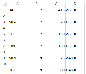
Image 6
Step 6: Delete Blank Rows and the Moneyline Column
To delete the blank rows:
- Select a cell in the first blank row (A2).
- While holding Ctrl, select one cell in each remaining blank row.
- Click the Delete dropdown arrow in the ribbon and choose Delete Sheet Rows.
Next, delete the Moneyline column (column C):
- Click the letter C at the top of that column.
- Click Delete → Delete Sheet Columns. (Note: When this is done, the Over/Under values will shift from column D to column C.)
Now it’s time to tidy up the Over/Under column by stripping out all lowercase o’s and u’s:
- Select column C and press Ctrl+H to open Find and Replace.
- In “Find what,” type a lowercase o, leave “Replace with” blank, then click Replace All.
- Repeat this process for lowercase u.
After both replacements, your cleaned-up Sheet2 should look like Image 7.

Image 7
Step 7: Merge Sheet2 Data into Sheet1
- In Sheet2, select all the cells that contain data and copy (Ctrl+C).
- Go to Sheet1, click cell B2, and paste (Ctrl+P).
You’ll now have your teams, spreads, and over/unders populated next to your formulas. Your spreadsheet should match what’s shown in Image 8 if you’re following along visually.
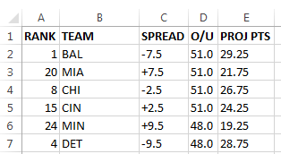
Image 8
Step 8: Sort the Spreadsheet by Rank and Over/Under
At this point, the RANK column won’t yet be in numerical order. We also want to sort secondarily by the Over/Under column (O/U) so that if two teams have the same rank, the team with the higher projected Over/Under appears first.
To sort in this manner, simply reference Image 9 and duplicate the settings shown in the Sort dialog box. It shows exactly what you need for a primary sort by RANK and a secondary sort by O/U.

Image 9
When you hit the ‘OK’ button to launch the sort, you might see a “Sort Warning.” That’s normal. Just choose the top option, “Sort anything that looks like a number, as a number,” and continue.
Once sorted, your table will list all teams in order of how many points Vegas projects them to score.
Step 9: Choose Your Kicker
That’s it! Your spreadsheet is now ready to help you make smarter kicker decisions.
- Simply select the first available kicker from the team at the top of the list, since teams near the top are projected to score the most points and typically have the most desirable fantasy kicker.
- Make sure the kicker you choose is active and healthy. For example, if he’s listed as doubtful or questionable on the injury report, consider picking the next available kicker on the list. And of course, if the kicker is listed as out for the upcoming game, you’ll need to find someone else.
For subsequent weeks, simply reuse the spreadsheet you’ve already created.
- Copy the new Vegas odds and clean them up using the process explained in this post.
- Paste the updated data into Sheet1.
Bazinga! Your rankings will automatically update and be ready for action each week.
Coming Up Next: Part 3 of 3
In the final post of this series, I’ll show you how to automate the entire process using AI, which can help recreate your kicker spreadsheet each week even more quickly. It’s the same system I use myself, and it’s surprisingly easy once it’s set up.
Stay tuned – Part 3 of 3 will take everything you’ve learned here and make it even faster and easier.
Leave a Reply
You must be logged in to post a comment.