Make a Fantasy Football Team Name Generator

Figure 1 – The Fantasy Football Team Name Generator interface
Making your own fantasy football team name generator is easy to do, and it’s entertaining to see the names that the program comes up with. As I mentioned in an earlier post, I would not recommend using a name generator to select a name for your team – using your creativity is still your best bet – yet the program may give you some ideas. But more than that, it’s mesmerizing simply to watch the multitude of combinations that the program constructs. Some names are clearly deficient, but every now and then it will generate a name that squarely hits the cool mark between the eyes.
(If you would prefer to simply use our team name generator rather than making your own, select ‘Team Name Generator’ from menu above, or click HERE.)
The name generator that I’ll show you how to make will randomly create a unique fantasy football team name from 10,000 possibilities with each push of a button. The only tools you’ll need are your computer and a typical spreadsheet such as Microsoft Excel or Apache OpenOffice Calc. In this post, I’ll show you how to make a fantasy football team name generator in both spreadsheets.
First I’d like to say a word or two regarding Excel and Calc. Excel is a great program with many strengths and a lot of flexibility. In fact, it is considered the industry standard for spreadsheets. But it’s not something the average person has installed on his/her computer because of the expense. That’s where Apache OpenOffice Calc shines. Calc can perform a lot of the same calculations, charts, and other duties as Excel, but without the price tag. Calc is free as part of the OpenOffice software suite, and if you don’t have a spreadsheet program installed on your computer, I would recommend that you download and install the OpenOffice software suite now. To learn more, check out www.openoffice.org. I have no affiliation with OpenOffice.org, but I consider the OpenOffice software suite one of FootballWebLog.com’s official software tools of choice.
Here’s a quick rundown on what the name generator does. It uses 100 descriptive words which, when the program is run, selects one of those words to randomly combine with one of 100 aggressive-sounding nouns. As an example, let’s say that one of the 100 descriptive words is “Fightin'”, and one of the 100 nouns is “Zombies”. If the program randomly selected those two words, the team name that would be generated would be “Fightin’ Zombies”. Make sense?
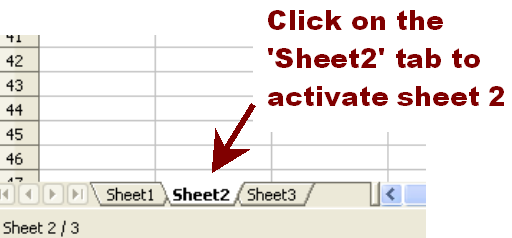
Figure 2
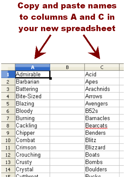
Figure 3
So let’s begin making the program. We’ll start by opening a new spreadsheet in Excel or Calc. Near the bottom of the spreadsheet, you’ll see three tabs that are created by default. The tabs are labeled ‘Sheet1’, ‘Sheet2’, and ‘Sheet3’. Click on the ‘Sheet2’ tab to activate sheet 2. (See figure 2.) Next, click on this link. When you do, an online spreadsheet will open that contains 100 descriptive words in column A, and 100 aggressive-sounding nouns in column C. Select/highlight all the words in column A and press Ctrl + C to copy the words to your computer’s clipboard. Now click in cell A1 of sheet 2 on your spreadsheet and press Ctrl + V to paste the words there. (See figure 3.) Go back to the online spreadsheet to copy the words from column C into column C of your spreadsheet using the same process.
Next we need to add a formula to the cells in columns B and D. To do this, we’ll start by entering the following text into cell B1 and hit the ‘Enter’ key:
=RAND()
Note that after you hit ‘Enter’, the cell will display a random decimal fraction between 0 and 1. If that happens, you’ll know you did it right. That’s exactly what we want.
Now copy the =RAND() formula to cells B2 through B100. A slick way to do this is to click on cell B1 to make it the active cell. Place the mouse pointer over the black square (fill handle) of the active B1 cell. The pointer will change to a plus (“+”) sign. Click and hold the left mouse button and carefully drag down until cells B1 through B100 are highlighted. (See figure 4.) (If at any time you mess up, just hit the undo button and try again.) Release the mouse button. Viola! The =RAND() formula now also exists in cells B2 through B100.
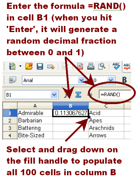
Figure 4 – Populate column B as explained in this figure. Repeat the procedure to also populate column D.
We next want to add the =RAND() formula to cells D1 through D100. To accomplish this, you can repeat the process we just used, or you can simply copy and paste the formulas from column B to column D.
You should now have four columns of information in sheet 2. Column A contains 100 descriptive words. Column C contains 100 aggressive-sounding nouns. Columns B and D each contain 100 cells with the formula =RAND().
Sheet 2 holds all of our data, and will be hidden from view when the finished program is used. Sheet 1 will be the interface that will display the randomly generated team names. Let’s move on to sheet 1.
The first things we want to do on sheet 1 are merge and justify some cells. This is done by selecting cells A4 through C4. Click on cell A4, hold down the shift key, and click on cell C4. Merge the selected cells by clicking on the ‘Merge Cells’ toolbar button along the top of the OpenOffice Calc screen. (The button is called ‘Merge and Center’ in Excel.) Merge cells D4 through F4 the same way. Lastly, right-justify the merged cell A4-C4 by making it active, and then clicking the ‘Align Right’ button located on the top of the screen. Repeat this procedure to left-justify the merged cell D4-F4 using the ‘Align Left’ button.
Alright, now we’re getting down to the nitty-gritty. The next thing we’re going to do is add two crucial formulas that make this program tick. The syntax for the formulas differs slightly between Calc and Excel, so make sure you enter the correct formulas for the program you’re using. It’s important that you enter the formulas exactly as shown.
OpenOffice Calc Spreadsheet
Enter the following in merged cell A4-C4:
=INDEX(Data.$A$1:$A$100;RANK(Data.B1;Data.$B$1:$B$100))
Enter the following in merged cell D4-F4:
=INDEX(Data.$C$1:$C$100;RANK(Data.D1;Data.$D$1:$D$100))
Microsoft Excel Spreadsheet
Enter the following in merged cell A4-C4:
=INDEX(Data!$A$1:$A$100,RANK(Data!B1,Data!$B$1:$B$100))
Enter the following in merged cell D4-F4:
=INDEX(Data!$C$1:$C$100,RANK(Data!D1,Data!$D$1:$D$100))
That’s it! The program should now be functional. Give it a try by hitting the F9 (calculate) key on your keyboard. Each time you press the F9 key, the program generates a new team name. If it’s not working, don’t panic. Look over the instructions again to make sure you didn’t miss anything. Double-check especially that the formulas on sheet 1 were entered correctly. My guess is that, if you’re having a problem, the most likely culprit will be a typo there.
So how does the program generate the names? I’ll try to explain. Every time you hit the F9 (calculate) key, each =RAND() formula on sheet 2 generates a new random decimal fraction. The formulas on sheet 1 use two functions to access those random decimal fractions: The RANK function, and the INDEX function. The RANK function looks at the first cell of each column of randomly generated decimal fractions, and determines its rank in ascending order among all the 100 numbers in the column. The INDEX function uses this rank number to display the associated word for that number. For example, if the decimal fraction of cell B1 is the 35th largest number value, then the 35th word in column A is used for the first half of the team name. Hopefully I’m not confusing you more than I’m helping. In all honesty, you really don’t need to know how the program works as long as it functions as intended.
Would you like to add your own descriptive words and nouns to the program? Feel free to do so. Just remember to tweak the formulas on sheet 1 as necessary. You’ll also need to make sure that you have a corresponding =RAND() formula for each word on sheet 2.
The final thing you may want to do is doll up the program to make it more attractive. Add some labels, tweak the color and sizes of text, change the background color, etc. It’s all your call. See figure 5 to see what I’ve done to the interface on my program.
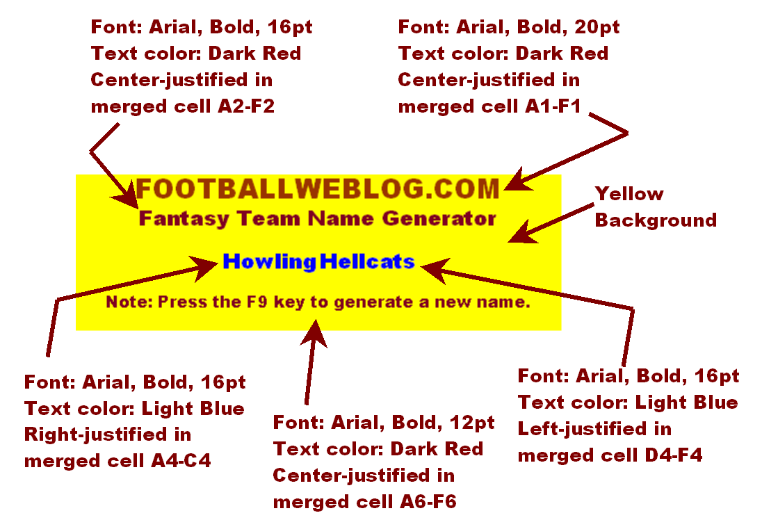
Figure 5
I hope you have fun with the program! Feel free to let me know if you have any questions.
As always, run to daylight!
~Randy